When the Schedule Becomes a Suggestion: Microgrid Flexibility with MPC
TL;DR — An energy-management system can plan a microgrid hours ahead, but its schedule will never match reality exactly. We designed a fast MPC layer that treats the plan as an informed reference—not an absolute command. A tuning weight determines how much freedom the controller has to depart from scheduled generator, storage, tie-line, and wind-curtailment setpoints when frequency or physical constraints require it.
A good plan becomes wrong in real time
Imagine that a microgrid’s energy-management system (EMS) has produced tomorrow’s operating plan. It schedules two thermal generators, a battery, a grid connection, and available wind power using long-horizon forecasts and market information.
Then operation begins:
- demand differs from the forecast;
- wind ramps earlier or later than expected;
- the battery reaches its energy limit;
- production costs change; or
- a generator becomes unavailable.
The schedule is still valuable: it contains information about expected renewable production, costs, commitments, and slow operational constraints. But following it exactly can allow an immediate power imbalance to move grid frequency.
Discarding it is equally wasteful. A fast controller should not rediscover a 24-hour unit-commitment plan every two seconds.
Our question was:
How can a fast frequency controller use a long-horizon EMS schedule while retaining enough freedom to correct the forecast errors and constraints that appear during operation?
Divide the problem by information and timescale
The proposed hierarchy separated two optimisation layers.
Energy-management system
The EMS handles the large, slow, and combinatorial problem. It can consider:
- day-ahead market decisions;
- unit switching and minimum-output requirements;
- long-term probabilistic demand and renewable forecasts;
- storage scheduling; and
- renewable curtailment.
The paper assumed at least a 24-hour forecast window with hourly granularity. Its output is a sequence of planned asset setpoints:
Model predictive controller
The MPC handles aggregated system dynamics on the scale of seconds. It observes frequency, estimates an unmeasured disturbance, incorporates short-horizon predictions, and calculates constrained control corrections.
Its output is the sequence actually requested from the controllable portfolio:
The important design choice lies between those two symbols. Must equal , or may it deviate?
Flexibility is permission to deviate
In this formulation, flexibility is not a single reserve number. It is the controller’s remaining ability to move each asset away from its planned reference while respecting:
- power limits;
- ramp-rate limits;
- battery state of charge;
- operational cost;
- forecast-informed targets; and
- supervisory decisions such as shutting down a unit.
The MPC objective combines frequency stabilisation with a portfolio term that penalises deviation from and accounts for asset costs.
One tuning parameter, , determines the balance:
- near , the MPC behaves mainly as a frequency regulator without the EMS-informed portfolio term;
- lowering gives the schedule and operational-cost terms more influence.
Within the portfolio term, additional weights balance reference tracking against general operating and deviation costs.
This means the EMS schedule is neither ignored nor enforced blindly. It acts as a soft contract: the controller pays an objective-function price for breaking it.
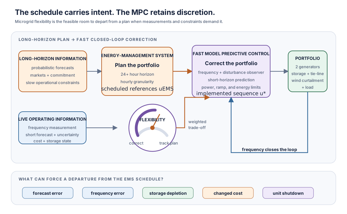
The EMS–MPC hand-off. Long-horizon forecasts and operational constraints produce an asset schedule. The fast MPC receives that schedule as a weighted reference, then spends the available flexibility when frequency measurements, short-term forecasts, storage state, costs, or supervisory constraints make deviation necessary.
Frequency closes the loop
The controller used a lumped swing-equation model to map active-power imbalance to deviation from nominal frequency. A Kalman filter estimated both:
- the aggregate dynamic state; and
- a residual disturbance representing the mismatch between intended and effective power balance.
From that disturbance estimate, the controller calculated an approximate stationary operating point. It could also combine the estimated past residual with a predicted short-term residual, weighted by their uncertainty.
That structure joins three sources of information:
- the EMS says where the portfolio was expected to operate;
- short-term prediction says what disturbance may be about to arrive;
- measured frequency reveals the imbalance that actually occurred.
The later target-adjusted MPC paper developed the equilibrium-adjustment aspect more directly. This conference paper’s distinctive focus was the broader EMS–MPC coupling and portfolio flexibility.
Storage changes flexibility over time
A generator’s power limit is not the same as a battery’s energy limit. A battery may be capable of delivering power now but unable to sustain it because its state of charge is nearly depleted.
The MPC updated storage constraints using:
- current stored energy;
- minimum and maximum charge;
- charging and discharging efficiency; and
- the control sampling interval.
As energy was charged or discharged, the feasible control region changed. Flexibility was therefore state-dependent: yesterday’s schedule could request an action that the battery could no longer provide.
Separating the storage-energy update from the main frequency model kept the online control problem manageable while still changing its constraints at each step.
The supervisory layer handles discrete events
Fast MPC used continuous control variables. Some portfolio decisions are discrete:
- start or stop a generator;
- enforce minimum up- or down-time;
- change the feasible operating range; or
- enable and disable resources.
A parallel supervisory layer dynamically reformulated the MPC constraints when such requirements changed. The EMS or supervisor owned the discrete decision; the MPC optimised within the resulting continuous feasible region.
This is another form of hierarchical responsibility: do not force a seconds-scale quadratic program to solve every market and commitment decision.
The constructed simulation
The illustrative portfolio contained:
- two thermal generators;
- one storage unit;
- a main-grid tie-line;
- a wind plant with controllable curtailment; and
- a time-varying load.
The controller sampled every two seconds and the quadratic programs were solved with Gurobi from a Python simulation. The chosen deliberately left the MPC substantial freedom to depart from EMS setpoints.
The scenario then introduced a sequence of operational events.
Demand ramps up
The load moved from zero to per unit. The controllable portfolio adjusted while frequency remained close to its reference.
Costs change
At timestep 1000, the first thermal generator became more expensive than the second. Its utilisation fell, demonstrating that the portfolio term could alter resource allocation for economic reasons.
The battery depletes
After the EMS changed references at timestep 1500, storage initially followed its request but eventually ran out of usable energy. The other assets had to replace its contribution.
Measurement disturbance appears
Random load noise was activated at timestep 2000. The disturbance observer and controller continued to reject its effect on frequency.
The wind schedule arrives early
The EMS changed its references in anticipation of increasing wind production, but the schedule moved before the wind ramp actually arrived. The MPC departed from the premature references to maintain balance, then brought the inputs back toward the plan after wind production increased.
A generator is shut down
Around timestep 3300, the supervisory system changed the constraints so that the second thermal generator was unavailable. The MPC redistributed the response among the remaining feasible assets.
Taken together, these events show what the paper meant by utilising flexibility: the controller could bend the planned portfolio trajectory without losing sight of it.
What was demonstrated
In the single simulation, the formulation simultaneously exhibited:
- frequency-reference tracking;
- rejection of load and renewable disturbances;
- tracking of EMS asset references when feasible;
- deliberate departure from those references under forecast error;
- changing dispatch in response to operational costs;
- hard power and ramp-rate constraint satisfaction;
- time-varying storage-energy constraints; and
- supervisory removal of a generator from the feasible portfolio.
The work did not compare the controller against PI, fixed-reference MPC, or another hierarchical architecture. It did not quantify an improvement in cost, renewable integration, frequency quality, or flexibility utilisation. The EMS itself was sketched as a stochastic-programming layer rather than evaluated jointly in a closed simulation.
The result was a controller formulation and a coherent proof-of-concept scenario—not evidence that it was universally better.
Where the uncertainty enters
It is tempting to describe this as “stochastic MPC,” but that would blur the division of labour.
- Long-horizon probabilistic scenarios belong primarily to the EMS.
- The MPC receives their effect indirectly through .
- Short-term disturbance forecasts and uncertainty can inform the fast controller.
- Frequency feedback corrects what neither forecast layer predicted.
The online optimisation shown in the simulation was a constrained quadratic program. It did not propagate a full long-term scenario tree every two seconds.
That separation was the computational point: keep the complex uncertainty problem slow enough to solve, and keep the dynamic correction problem fast enough to control.
Limitations
- One illustrative simulation. There was no statistical evaluation over many forecasts or disturbances.
- No baseline controller. Relative performance and value of information were not measured.
- Assumed EMS output. The long-horizon stochastic layer was described but not jointly validated.
- Aggregated linear model. Voltage, network flows, spatial constraints, and detailed nonlinear plant behaviour were omitted.
- Tuning dependence. The apparent flexibility depends strongly on and the portfolio weights.
- Observer and forecast dependence. Incorrect disturbance dynamics or overconfident short-term predictions can degrade control.
- Simplified storage. The state update represented charge, efficiency, and standing loss without detailed battery aging or thermal limits.
- Simulation only. Communication, computation deadlines, and equipment interfaces remained untested.
The paper also identified robustness of the EMS–MPC coupling, indirect control of additional flexibility, critical operating conditions, and voltage-angle control as future work.
The broader lesson
A hierarchy is useful when each level sends the next level not just a command, but a statement of intent with room for correction.
The schedule carries long-horizon knowledge. Feedback carries reality. MPC is the negotiation between them.
For further reading
- Original paper: Banis, Guericke, Madsen, Poulsen, “Utilizing flexibility in Microgrids using Model Predictive Control,” MEDPOWER 2018. DOI: 10.1049/cp.2018.1856
- Publication record: Utilizing flexibility in Microgrids using Model Predictive Control
- Related project: Target-Adjusted MPC for Microgrid Frequency Control
- Later journal explainer: Move the Equilibrium, Not the Frequency
- Laboratory hierarchy explainer: When the Schedule Meets the Grid