Control Without Command: Using EV Prices to Support a Microgrid
TL;DR — Electric vehicles can help balance a microgrid without surrendering direct control of their batteries. The microgrid sends an economic incentive, observes the aggregate charging response, and updates a time-dependent response model. A redispatch layer then coordinates that uncertain, slower flexibility with fast directly controlled generation. In simulation, price-responsive charging partly absorbed disturbance steps—but the EV behaviour was synthetic and deliberately simplified.
Flexibility without taking the keys
An electric vehicle can be useful to the power system while it is plugged in. Charging can be delayed, reduced, or increased to help match uncertain renewable production.
One way to access that flexibility is direct control: give a central controller authority over the charger. That produces a clear command–response channel, but it requires communication infrastructure and restricts the owner’s autonomy.
Indirect control takes a different approach:
- the microgrid offers a price or reward;
- each EV controller decides how to respond;
- the microgrid observes only the aggregate change; and
- the control system learns how price maps to power.
The attraction is practical and institutional: owners retain decision authority. The difficulty is technical:
A price is not a command.
The response depends on time of day, battery charge, planned journeys, owner preferences, and the local charger controller. It can be delayed, uncertain, and different tomorrow.
Our question was:
Can a microgrid learn this changing price response online and coordinate it with directly controlled assets to support real-time power balance?
Four layers, four timescales
The proposed hierarchy assigned different responsibilities to different update rates.
Energy-management system: approximately hourly
The EMS considered day-ahead and real-time market bids, uncertain production and consumption, storage, and renewable curtailment. Its 24-hour schedule became a reference for real-time operation.
Redispatch: every 1–15 minutes
Redispatch co-optimised:
- directly controllable units, such as generation; and
- indirectly controllable prosumers, such as price-sensitive EV charging.
It could emphasise economic performance or robustness, depending on the operating situation. Its output became a reference for both control channels.
Direct control: every 1–5 seconds
Fast direct control handled frequency stabilisation. An extended-state observer estimated an unmeasured power disturbance, and a quadratic controller tracked the redispatch reference while respecting power and ramp-rate constraints.
Indirect control: every 60–600 seconds
The indirect controller chose a price intended to produce a desired aggregate EV response. It operated more slowly because the vehicles needed time to react and because their response had to be identified statistically.
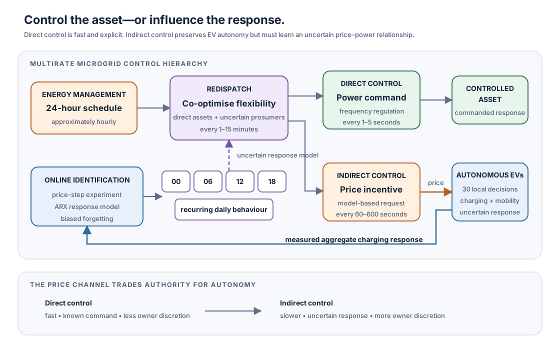
The control-without-command hierarchy. The EMS supplies a long-horizon schedule; redispatch coordinates directly controlled assets with an uncertain aggregate EV response. Fast direct control acts in seconds, while indirect control sends a price and observes EV charging over minutes. Online identification updates an hour-specific response model for the next redispatch decision.
This hierarchy reflects a physical asymmetry. A generator setpoint can change within seconds. A population’s response to an incentive is slower and less certain. Treating both as identical actuators would hide the most important part of the problem.
Redispatch with two kinds of actuator
During normal co-optimisation, redispatch could choose both:
- : inputs to directly controlled units;
- : desired responses from indirectly controlled units.
The objective balanced operating cost against violations of power-balance or output limits. Direct units entered with known constraints and costs. EV flexibility entered through an estimated response model and therefore carried additional uncertainty.
During a system-identification event, the price had to remain fixed long enough for the EV response to settle. The desired indirect input was then treated as a parameter rather than a redispatch degree of freedom. Direct assets carried the remaining balancing responsibility.
That is an important operational cost of learning: an experiment temporarily restricts what the controller is free to change.
Turning a price into a predicted response
The indirect-control problem selected a price sequence whose predicted aggregate response followed the response requested by redispatch:
The first term rewards matching the desired flexibility. The second discourages excessive departure from a reference price.
The mapping from price to response was represented by an estimated model for the currently active temporal cluster . An autoregressive model with an exogenous price input was one proposed structure.
The controller therefore did not assume “one euro always buys one kilowatt.” It asked a narrower question:
At this time, given recently observed behaviour, what response distribution should this price produce?
Why the clock belongs in the model
EV charging behaviour has a daily rhythm. Cars arrive, charge, and depart at characteristic times. The simulated aggregate state of charge was highest in the early morning and lowest in the afternoon.
A single all-day response model mixes fundamentally different operating conditions:
- many connected batteries with spare capacity;
- few available vehicles;
- batteries already near full charge;
- periods dominated by driving.
The paper therefore organised identified models into:
- daily meta-clusters; and
- hourly clusters within each day.
Models collected around the same recurring hour informed the active price-response estimate. Comparing one hour-specific cluster with a collection of many hourly clusters showed much greater spread in the latter. That supported temporal clustering: apparent uncertainty can come from pooling different behavioural regimes.
Learning online—and forgetting selectively
A system-identification event began when the price changed by more than a threshold. The price was then held constant for a chosen settling time while the aggregate response was recorded.
Newly identified model parameters were added to the relevant temporal cluster. To keep the cluster finite and adaptive, old parameter sets had to be removed. The study used biased forgetting: once a cluster exceeded its size limit, the parameter set furthest from the cluster median was removed. This keeps the model concentrated around recent typical behaviour and can improve prediction when operating conditions drift. It also has a serious statistical implication:
- outlying responses may be obsolete or erroneous;
- but they may instead be real rare behaviour;
- removing them narrows the estimated uncertainty by construction.
The resulting confidence should therefore be interpreted as confidence in a trimmed behavioural model—not automatically as calibrated tail risk.
The simulated EV population
The numerical example contained:
- one directly controllable first-order unit;
- 30 simulated EVs;
- nominal EV charging power of approximately 3.6 kW per vehicle;
- battery capacity of approximately 24.2 kWh per vehicle;
- first-order charging-response dynamics with a roughly 180-second time constant; and
- 216 kW nominal total microgrid consumption.
At nominal conditions, the EV fleet represented about half of that power. The unexcited charging and state-of-charge patterns were generated over recurring daily operation. The assumed steady-state response to price was linear within saturated upper and lower bounds. This was not an empirically identified fleet model. It was a synthetic population chosen to exercise the control and identification architecture.
What the simulations showed
The paper first examined response estimation:
- a single hour-specific cluster produced a relatively concentrated aggregate response;
- pooling many hourly clusters produced considerable variation; and
- temporal clustering retained the recurring time dependence that an all-day model would smear out.
It then compared two control cases:
- DC: fast directly controlled power only;
- DC + IC: direct control supported by price-responsive EV charging.
When a disturbance step arrived, indirect EV response partly compensated it. The directly controlled unit consequently needed a smaller power step, and the frequency trajectory changed accordingly.
A second example allowed the simulated charge interaction to evolve while price was used to reduce the effect of multiple disturbance steps. Again, the result illustrated partial support rather than perfect cancellation.
The central evidence is qualitative:
Adding an indirectly controlled, price-sensitive load can reduce the balancing burden placed on a directly controlled asset.
What was—and was not—established
The study demonstrated a coherent simulation architecture in which:
- a long-horizon schedule flows into redispatch;
- redispatch co-optimises direct and indirect flexibility;
- fast direct control stabilises frequency;
- a slower price signal activates EV charging response;
- online experiments update the response model; and
- temporal clusters represent recurring time variation.
It did not establish:
- response accuracy on measured EV data;
- calibrated uncertainty or rare-event coverage;
- owner acceptance of the incentives;
- economic savings or optimal incentive levels;
- rebound-free charging in a real fleet;
- network-feasible charging at individual locations; or
- closed-loop stability guarantees for the complete multirate hierarchy.
The missing rebound
The assumed price-response curve reduced or increased charging within saturation bounds, but it did not model rebound.
In reality, energy not charged now may have to be charged later before departure. A price signal can therefore move demand rather than eliminate it. Ignoring rebound can make short-term flexibility look larger and cheaper than it is across the full day.
Likewise, an aggregate response says little about whether individual owners meet their departure state-of-charge requirements. Those issues require a richer mobility and energy model.
Limitations
- Synthetic population. Vehicle behaviour and price sensitivity were assumed rather than learned from field data.
- Only 30 EVs. Scaling, diversity, and aggregation effects were not established.
- Simplified linear response. Saturation was included; rebound and owner-level constraints were not.
- Qualitative comparison. The figures did not report summary performance metrics or repeated trials.
- Biased uncertainty. Selective forgetting deliberately removes the largest parameter excursions.
- Identification requires excitation. Price steps must be sufficiently large and held long enough to observe a response.
- Central data architecture. Privacy, communication loss, cybersecurity, and strategic behaviour were outside scope.
- Timescale interaction. Stability and robustness of all coupled layers require further analysis.
The broader lesson
Indirect control changes what “control” means. The system does not dictate an action; it shapes an incentive, observes a population, and revises its belief.
This is a feedback loop through human-mediated assets. Its value lies in preserving autonomy; its cost is uncertainty. A responsible controller must model both.
For further reading
- Original paper: Banis, Guericke, Madsen, Poulsen, “Supporting power balance in Microgrids with Uncertain Production using Electric Vehicles and Indirect Control,” IFAC-PapersOnLine 52(4), 2019. DOI: 10.1016/j.ifacol.2019.08.238
- Publication record: Supporting power balance using electric vehicles and indirect control
- Related market explainer: A Thousand Batteries, One Bid
- Related MPC explainer: When the Schedule Becomes a Suggestion
- Related identification explainer: Sparse First, Bayesian Second