Sparse First, Bayesian Second: Learning Prosumer Dynamics with SINDYc and MCMC
TL;DR — SINDYc searches a library of candidate terms for a compact dynamical model. That sparse model can then focus Markov-chain Monte Carlo (MCMC) on a smaller, better-posed parameter space. In our synthetic prosumer study, the combination recovered useful model structure and produced probabilistic simulations—but it also exposed an essential warning: Bayesian output is not automatically well calibrated. Experiment design, the candidate library, the forcing model, and the prior still determine what can be learned.
A controller needs more than a response curve
A prosumer can both consume and supply electricity. An electric vehicle with vehicle-to-grid capability, for example, may charge when prices are low and return power when the grid needs support.
To coordinate many such resources, an operator needs a model of their response to an incentive. A static statement such as “demand falls when price rises” is not enough. Timing matters: how quickly does the response develop, how long does it persist, and how much does it vary?
Those dynamics are difficult to specify from first principles when the internal equipment and preferences of each prosumer are unknown. System identification offers another route: excite the system, observe its response, and infer a dynamical model from the data.
But a useful operational model has to answer two separate questions:
- Which mathematical terms belong in the dynamics?
- How uncertain are their coefficients and predictions?
Our study connected two methods to address those questions in sequence.
First find a sparse model
SINDYc—Sparse Identification of Nonlinear Dynamics with control—assumes that the observed dynamics can be described using only a few terms from a larger candidate library.
For a state driven by a price signal , the general idea is:
is the library of possible terms; contains their coefficients. In this study the library was a polynomial expansion, including state terms, price terms, and their interactions. The candidate response model was restricted to:
Sequential thresholded least squares removes coefficients whose contribution is too small. Sweeping the regularisation strength produces candidate models with different levels of sparsity.
The desired outcome is not simply the model with the fewest terms. It must also remain stable and reproduce the observed dynamics over the intended operating range. Sparsity is therefore a filter on model complexity, not proof that the discovered equation is physically true.
Then infer parameter distributions
SINDYc normally returns coefficient estimates. It does not, by itself, provide a posterior distribution over those coefficients.
The second stage uses a selected SINDYc model to construct the Bayesian model:
- zeroed SINDYc terms are omitted from the sampling problem;
- retained SINDYc coefficients inform the prior means;
- prior widths express the assumed uncertainty around those coefficients; and
- MCMC samples the posterior using the observations and likelihood.
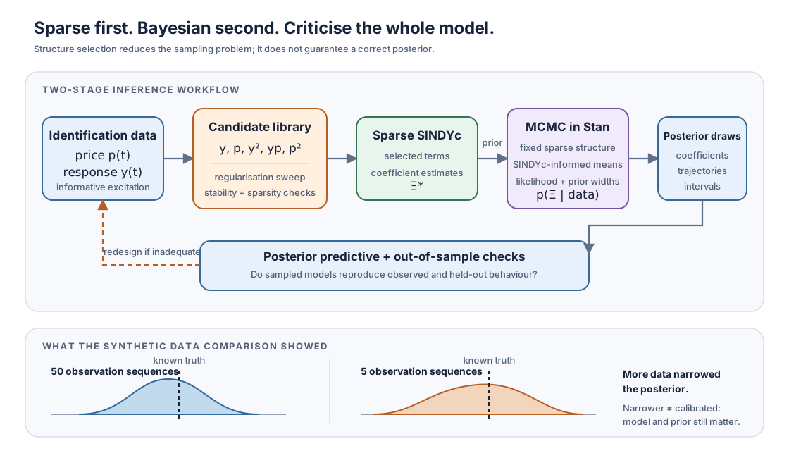
The two-stage workflow. SINDYc uses an excitation experiment to select a sparse candidate structure. That structure and its coefficients focus the prior used by MCMC. Posterior predictive checks and out-of-sample simulations then test the complete probabilistic model—not just the fit of its mean.
This division of labour is the central idea:
SINDYc reduces the structural search space; MCMC characterises uncertainty within the selected structure.
The sparse first stage may reduce the computational burden of the sampling stage. It does not guarantee that the selected structure, prior, or posterior is correct.
The demonstration
The paper used a deliberately simple synthetic system of two prosumers:
- one had nonlinear dynamics;
- the other had linear dynamics;
- both responded to a scalar price signal;
- process and measurement noise were added; and
- the system was sampled once per second.
Because the data were simulated, the true equations and parameter distributions were known. This made it possible to inspect not only whether the inferred model reproduced a trajectory, but whether its coefficients agreed with the system that generated the data.
A two-frequency sinusoidal price signal excited the system after a burn-in period. Two data regimes were compared:
- cluster : 50 independent observation sequences;
- cluster : 5 independent observation sequences.
This was an illustrative identification problem, not a field trial with household, battery, or electric-vehicle measurements.
What SINDYc recovered
With a sufficiently informative excitation signal, the sparse-identification stage distinguished the nonlinear prosumer from the linear one and produced low-order candidate models. The nonlinear candidate reproduced the simulated response both on identification data and under a separate out-of-sample excitation.
The comparison between 50 and 5 observation sequences showed the expected data effect: coefficient estimates varied more in the smaller-data cluster.
But the success depended on the excitation. A sparse model was recovered only when the price signal made the relevant dynamics visible. If an experiment never explores a region where a nonlinear term matters, no selection algorithm can reliably identify that term.
This is a foundational system-identification lesson:
Data volume matters, but informative excitation matters first.
What MCMC added—and what it did not
The selected nonlinear SINDYc model supplied a reduced candidate structure and prior means for inference in Stan. The No-U-Turn Sampler generated posterior distributions over the retained coefficients. As expected, the posterior was narrower for the 50-sequence cluster than for the five-sequence cluster.
Those distributions enabled:
- intervals over model coefficients;
- random parameter draws;
- posterior predictive checks; and
- probabilistic out-of-sample simulations.
This is more informative than returning one coefficient vector. It exposes how parameter uncertainty propagates into possible system trajectories.
However, the known synthetic truth also revealed shortcomings:
- the inferred posterior distributions deviated from the true parameter distributions;
- the SINDYc coefficient means were closer to the true means than the inferred posterior parameters in the reported example;
- posterior predictive checks captured the general output trend only sub-optimally; and
- the third-order polynomial model used to represent the excitation signal introduced additional loss of precision.
It would therefore be inaccurate to say that the study demonstrated calibrated uncertainty. It demonstrated a workflow for obtaining parameter distributions—and, just as importantly, showed how a plausible Bayesian workflow can remain misspecified.
Why the sparse prior is powerful
Sampling every conceivable polynomial term would enlarge the parameter space and spend computation on terms that the identification stage has already judged uninformative. By passing a parsimonious candidate model into MCMC, the workflow concentrates sampling on a smaller set of coefficients.
That has two potential benefits:
- fewer parameters can improve sampling efficiency and convergence;
- the prior can encode a concrete, data-informed candidate rather than starting from an unrestricted library.
But using SINDYc twice—first to choose the terms and then to centre the priors—also makes its errors consequential. If it omits a real term, MCMC cannot recover that term because it is no longer in the model. If its coefficient estimates are biased, prior design determines how strongly that bias carries into the posterior.
The pipeline is therefore best understood as a disciplined hand-off, not an automatic truth machine.
Four checks that determine whether to trust the result
1. Was the system excited informatively?
The input must cover the amplitudes and frequencies at which the model will be used. Normal operation may constrain how aggressively a real prosumer can be probed, motivating safer active-learning designs.
2. Was the right candidate library available?
SINDYc can only select terms it is offered. Polynomial libraries are convenient and broad, but their size grows rapidly with dimension and their extrapolation can be poor. Domain knowledge should shape the library.
3. Does the prior help without over-constraining?
A SINDYc-informed prior can focus inference, but its width must admit plausible departures from the initial coefficient estimate. The paper’s results indicate that the chosen prior formulation deserved further refinement.
4. Does the probabilistic model predict held-out behaviour?
Trace plots and narrow intervals are not enough. Posterior predictive checks and out-of-sample excitation tests ask whether draws from the inferred model reproduce the observations and generalise to a different experiment.
What the study established
The paper’s contribution was a first investigation of coupling SINDYc with MCMC for prosumer-response modelling. It established that:
- a sparse SINDYc candidate can define a constrained parameter space for Bayesian inference;
- linear and nonlinear synthetic response structures can be distinguished under informative excitation;
- data availability changes the width of inferred parameter distributions;
- the resulting posterior can drive probabilistic simulations; and
- the complete workflow is highly sensitive to experimental and probabilistic-model design.
The probabilistic model was motivated by possible downstream use in stochastic MPC, where uncertainty can be propagated into constrained decisions. That use was prospective; the paper did not validate a controller driven by the inferred posterior.
Limitations and next steps
- Synthetic demonstration. Evaluation on measured prosumer or demand-response data remains necessary.
- Small system. The example contains two low-dimensional prosumers, not a large heterogeneous population.
- Hand-designed excitation. The double-sinusoidal price signal was selected naively rather than optimised subject to operational constraints.
- Restricted polynomial library. Higher-dimensional systems would face combinatorial growth and potentially weak extrapolation.
- Imperfect forcing model. Stan required a model of the excitation signal; the selected third-order polynomial approximation reduced precision.
- Sub-optimal posterior fit. Neither a Bayesian label nor a 95% interval establishes calibration. Prior and likelihood design require validation.
- Structural uncertainty is not propagated. MCMC samples coefficients within one selected structure; uncertainty over alternative SINDYc structures is not integrated.
We may describe the methodological pattern as:
The final step is indispensable. An interpretable equation and a posterior distribution make a model easier to inspect; they do not exempt it from falsification.
For further reading
- Original paper: Banis et al., “Prosumer Response Estimation Using SINDYc in Conjunction with Markov-Chain Monte-Carlo Sampling,” Energies, 2020. DOI: 10.3390/en13123183
- Open-source implementation: SINDYc and MCMC Framework (Zenodo, v1.1.1)
- Related project: SINDYc and MCMC for Prosumer Response Estimation
- Publication record: Prosumer Response Estimation Using SINDYc and MCMC
- Research trajectory: From Energy Grids to Adaptive Biomedical Sensing