When Adaptive Sensing Doesn’t Win (And Why That’s Interesting)

TL;DR — Adaptive sensing sounds like it should always win: measure where you’re most uncertain, reduce error faster, done. On two controlled toy problems, it didn’t work that way. A 1D radar-like reconstruction toy showed that posterior variance is noise-dominated and cannot rank locations by error. A 2D point-source tomography toy showed that greedy policies converge 30–60% faster early but random selection catches up because greedy choices reduce geometric diversity. The negative results are informative — they map the boundary conditions where adaptive sensing earns its keep and where it doesn’t.

What Is Adaptive Sensing, and Why Would You Expect it to Work?

The idea is simple. You have a physical system you want to reconstruct — a radar field, a tomographic image, a temperature distribution — but measurements are expensive, noisy, or limited. Rather than measuring uniformly and hoping for the best, you let the system decide where to measure next based on its current uncertainty. Measure where the posterior variance is highest, update your belief, repeat. In principle, this concentrates the measurement budget where it carries the most information, converging faster than blind uniform sampling.

This is the promise of uncertainty-driven acquisition: treat measurement selection as a sequential decision problem, use the current posterior to estimate where uncertainty is largest, and choose the next measurement to maximise information gain. It connects to a rich theoretical literature on Bayesian optimal experimental design, active learning, and information-theoretic acquisition. The machinery is principled and well-motivated.

So when we ran two toy experiments to test it, we expected adaptive policies to beat naive baselines. They didn’t — at least, not consistently. The story of why is more interesting than a simple win or loss.

Toy 1: 1D Radar-Like Signal Reconstruction

The Setup

The first toy simulates respiratory motion estimation from noisy radar-like phase measurements. A synthetic phase time-series is generated from a known respiratory signal (sinusoidal with harmonic distortion), and Gaussian noise is added at SNR levels of 10, 20, and 30 dB. A Bayesian linear regression model with physics-informed basis functions (Fourier + cardiac harmonics) recovers the signal and produces posterior predictive uncertainty.

The adaptive sensing question: can we use the posterior variance to decide which time points to sample next, and does that beat uniform sampling?

What Happened

The posterior variance is noise-dominated. Across all SNR levels, the model-variance fraction — the share of predictive uncertainty coming from epistemic uncertainty rather than the noise term — is about 0.9%. The posterior standard deviation is nearly constant across time points. It cannot rank locations by error because it barely varies.

This is a fundamental problem for uncertainty-driven acquisition: if your uncertainty estimate is flat, selecting the “most uncertain” location is no better than selecting randomly. The experiment confirmed this directly. We tested five sampling policies — uniform, random, posterior-variance-driven, ensemble-disagreement-driven (bootstrap Bayesian LR), and a hybrid — across 50 Monte Carlo trials per condition. No adaptive policy consistently beats uniform sampling.

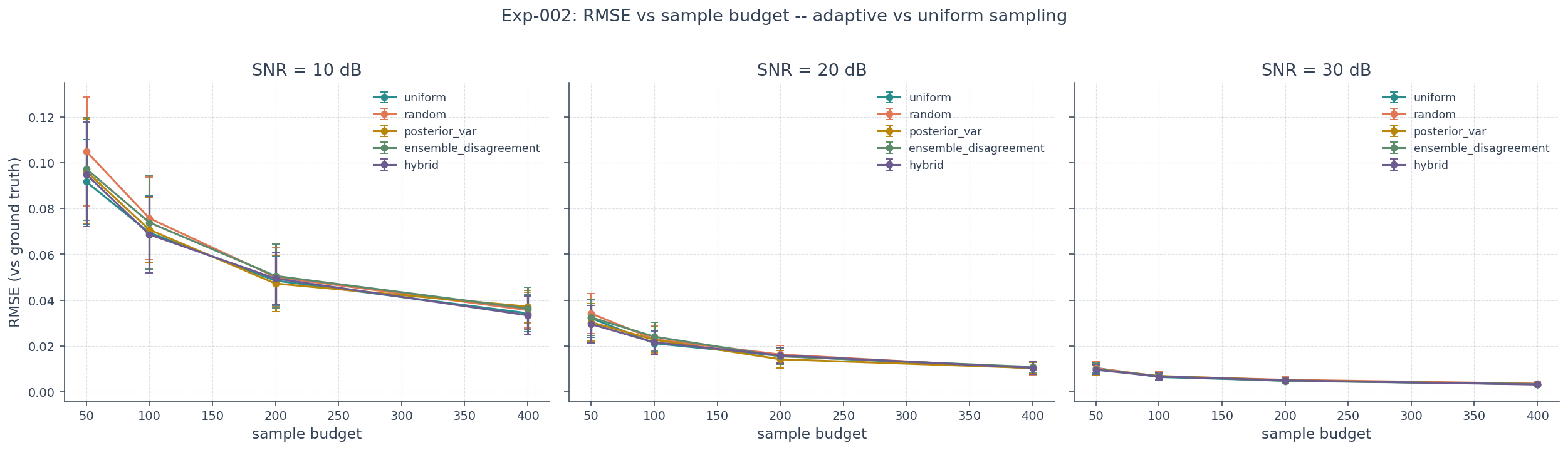Figure 1: RMSE vs sample budget for all five sampling policies on the 1D radar-like toy. No policy is reliably best; uniform sampling is a strong baseline.

Why: The Basis Function Has Global Support

The deeper reason is structural. The Bayesian linear regression uses a global Fourier basis. Each time point contributes similarly to the global fit because every basis function has support across the entire domain. There is no localised epistemic uncertainty for adaptive sampling to exploit — the model doesn’t “know more” in one region than another, because every measurement informs all basis coefficients equally.

Ensemble disagreement doesn’t help either. We tested bootstrap-resampled Bayesian LR models, expecting their disagreement to track true error. It doesn’t: the correlation between ensemble disagreement and true error is negative (r = -0.363 at SNR=20 dB). Single-model posterior variance has zero correlation. Neither metric can guide acquisition.

The lesson: uncertainty-driven acquisition requires an uncertainty signal that actually varies across candidate measurements and correlates with error. A global basis with noise-dominated posterior variance provides neither.

Toy 2: 2D Point-Source Tomography

The Setup

The second toy is richer. A 2D point source is hidden in the plane, and the measurement device chooses a projection angle and observes a noisy 1D projection. After each measurement, the system updates its belief about the source location and selects the next angle. We compare four acquisition policies:

1. random — random angle selection without replacement
2. uniform — evenly spaced angles
3. projected_var — greedily pick the angle maximising projected posterior variance (a_i^T Sigma a_i)
4. info_gain — greedy expected information gain (0.5 * log(1 + a_i^T Sigma a_i / sigma^2))

We used the analytic Gaussian posterior (exact, not a trained EBM) to isolate the policy question from inference quality. 200 Monte Carlo trials per policy. Two configurations: a standard setup (8 angles, 6 measurements) and a harder one (16 angles, 8 measurements).

What Happened: Faster Early, Random Catches Up

Here adaptive sensing does work — but only partially. In the first 4 measurement steps, the greedy policies (projected_var and info_gain) have 30–60% lower RMSE than random and uniform. The adaptive policies are very effective at reducing uncertainty early. This is the result the theory predicts.

But by the final steps, random overtakes the greedy policies. In the standard configuration, random wins with RMSE 0.1025 vs projected_var at 0.1125 (worst). In the hard configuration, random wins again at 0.0912, with uniform worst at 0.1072. The adaptive advantage evaporates as the measurement budget grows.

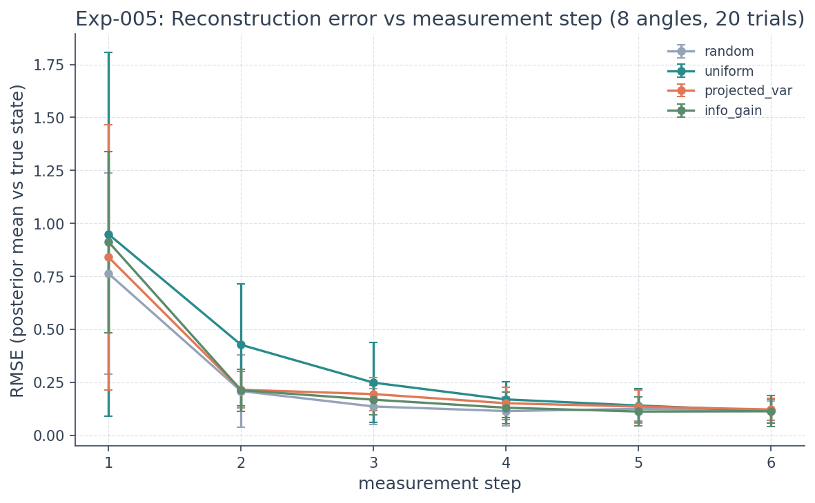Figure 2: RMSE vs measurement step per policy on the 2D point-source toy. Adaptive policies (proj_var, info_gain) dominate early; random catches up by the final steps.

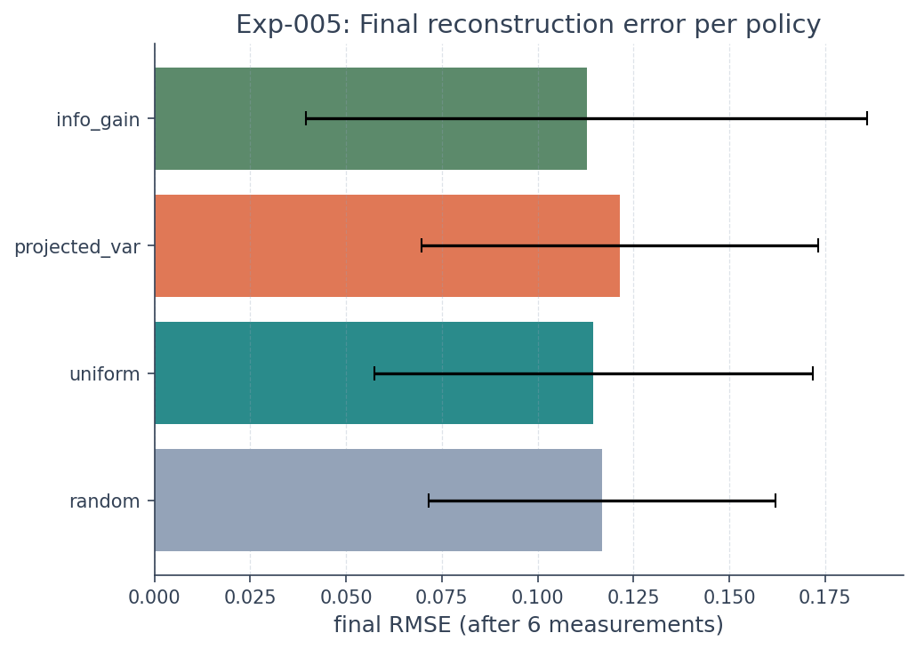Figure 3: Final RMSE per policy on the 2D point-source toy (standard config). The spread is only 8.9% — no decisive winner.

The Geometric Intuition: Why Greedy Clusters

The reason random catches up is geometric. Greedy angle selection picks the direction of maximum projected variance. After measuring along that direction, the variance in that direction shrinks — but the next most uncertain direction is often close to the same axis, because the posterior is elongated along the axis orthogonal to the first measurement. The greedy policy tends to cluster measurements in similar directions, reducing the geometric diversity of the measurement set.

Random selection, by contrast, naturally explores the full angle space. Each random measurement tends to cover a new direction. As the budget grows, the geometric diversity of random sampling pays off: the posterior is constrained from all sides, and the error drops below the greedy policies that have been re-measuring similar directions.

This is a known failure mode of greedy acquisition: it exploits locally but doesn’t explore globally. The information-theoretic literature has proposed fixes — UCB-style exploration bonuses, Thompson sampling, mixed strategies — but in our toy, a mixed strategy (adaptive early, random late) does not dominate either. It performs between its pure counterparts, improving over pure projected_var but never beating the best pure policy.

Which Acquisition Rule Wins?

A subtler finding: info_gain is consistently the best or near-best policy, even when random beats projected_var. In the standard config, info_gain (0.1041) beats random (0.1091) by 4.5%. In the hard config, info_gain (0.0928) beats random (0.0947) by 2.0%. The log-formula of information gain appears to regularise the greedy choice slightly, avoiding the worst clustering behaviour of raw projected variance.

A learning could be: if you must choose a single greedy rule, use information gain, not projected variance.

When Does Adaptive Sensing Actually Win?

The two toys above are deliberately simple — and that simplicity is exactly why adaptive sensing doesn’t shine. The 1D toy has a global basis with noise-dominated uncertainty. The 2D toy has a Gaussian posterior in low dimensions with a comfortable measurement budget. In both cases, the structure that adaptive acquisition exploits — spatially varying epistemic uncertainty, scarce measurements relative to state dimensionality — is absent.

A follow-up scaling experiment (extending the 2D toy to D = 2, 4, 8, 16 hidden dimensions) confirmed the pattern: adaptive sensing wins decisively when the measurement budget is tight relative to state dimensionality. At D=16 with a tight budget (D+2 measurements), info_gain beats random by 31.6%. At the same dimensionality with a comfortable budget (2*D measurements), the advantage shrinks to 2.9%.

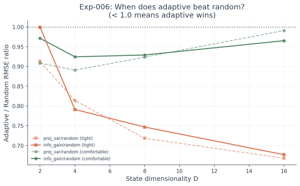Figure 4: Adaptive-to-random RMSE ratio vs state dimensionality. Lower is better for adaptive. At the tight budget (D+2), the advantage grows from 2.4% at D=2 to 31.6% at D=16.

This maps out the boundary conditions:

Condition	Adaptive Helps?	Why
Global basis, noise-dominated uncertainty	No	Uncertainty signal is flat, cannot rank locations
Low-dimensional posterior, comfortable budget	Marginal / no	Random covers the space well enough
Low-dimensional posterior, tight budget	Small advantage	Greedy reduces early uncertainty faster
High-dimensional posterior, tight budget	Yes, decisively	Random cannot cover the space; greedy concentrates scarce measurements where they matter

What This Means for the Field

The broader lesson is about the gap between theoretical expectations and empirical results in uncertainty-aware ML. Adaptive sensing is theoretically motivated by information-theoretic arguments that assume the uncertainty estimate is well-calibrated, varies meaningfully across candidate actions, and the measurement budget is scarce relative to the problem’s information content. When those assumptions hold, adaptive works. When they don’t — when the uncertainty is noise-dominated, the posterior is low-dimensional, or the budget is comfortable — the theoretical advantage evaporates and naive baselines are hard to beat.

The negative results are productive because they tell us when to invest in adaptive acquisition and when a simple uniform or random baseline is sufficient. In practical settings — clinical imaging with dose constraints, adaptive microscopy with phototoxicity limits, sparse-angle CT — the budget is genuinely scarce, and the state space is high-dimensional. That is where adaptive sensing should earn its keep.

Connection to the Research Direction

These experiments are part of a broader program in mechanistically grounded ML for adaptive biomedical sensing. The three complementary threads — physics-informed neural networks for reconstruction, energy-based models for adaptive measurement, and solver-coupled training for physical validity — converge on a vision of closed-loop experimental systems that infer, decide, and act under uncertainty.

The negative results sharpen the research agenda. They tell us:

1. We need harder problems. The 2D point-source toy is too simple to show a decisive adaptive advantage at convergence. Higher-dimensional problems with tight budgets are where the value lies — and where we now have positive evidence.
2. We need better uncertainty metrics. Posterior variance from a single model with a global basis is noise-dominated and useless for acquisition. Ensemble disagreement is anti-correlated with error. The next step is to test whether a trained energy-based model (EBM) posterior — which can represent non-Gaussian, multi-modal distributions — provides a richer uncertainty signal for adaptive selection.
3. Information gain beats projected variance as the acquisition rule. This is a small but actionable finding for anyone implementing adaptive sensing: the log-formula regularises the greedy choice and avoids the worst clustering behaviour.

The Methods page describes the four pillars — uncertainty-aware inference, adaptive decision-making, closed-loop experimentation, and mechanistic ML — that frame this work. The Research page situates it in the broader program of uncertainty-aware modelling for systems that must infer, decide, and act under imperfect information.

Limitations

All results are from controlled toy problems with synthetic data and known physics. The 2D tomography toy uses an analytic Gaussian posterior, not a trained EBM — so the policy comparison isolates the acquisition rule from inference quality. Whether the findings transfer to real-world biomedical sensing (mmWave radar, sparse CT, adaptive microscopy) remains an open question. The scaling experiment suggests the direction is promising, but the EBM posterior may introduce additional noise that changes the picture. We’re testing that next.

---

Follow-up: Mixed Acquisition Strategies (2026-07-05)

After publishing this post, we ran a follow-up experiment (experiment log exp-physically-grounded-ml-blog-002) testing four families of exploration-aware policies designed to counteract the geometric clustering described above:

1. Adaptive early / random late with three tuned switch points.
2. UCB-style exploration bonuses on the information-gain score, with two bonus coefficients.
3. Thompson sampling over the posterior (stochastic picks that preserve uncertainty instead of taking the argmax).
4. Diversity-aware selection that penalises candidate angles close to already-measured angles, with two penalty coefficients.

The result was a clean negative: no mixed strategy significantly dominates the best pure baseline on any setup (2D toy or the D=2/4/8/16 tight-budget scaling sweep, 200 paired Monte Carlo trials, paired Wilcoxon signed-rank test at alpha=0.05). The UCB and diversity-aware policies produced small (1.5-4.5%) point-estimate improvements at D=2/4/8 but none reached significance, and at D=16 the pure info_gain policy won outright. The naive switch family was the worst mixed family at every D >= 4, confirming that the exp-005b finding generalises: switching from adaptive to random at a fixed step throws away the greedy exploitation that matters most when the budget is tight.

The diversity metric showed that the greedy info_gain policy already achieves high angular diversity on the linear-Gaussian toy – the clustering failure mode identified in this post is real but small enough that the exploration bonuses do not help. The natural next test is a non-Gaussian posterior or a harder forward model where greedy clustering is more severe, which is outside the scope of this follow-up.

The negative finding strengthens the message of this post: on controlled toy problems with the analytic Gaussian posterior, the obvious fixes for greedy clustering do not rescue mixed strategies. The value of adaptive sensing remains in the regime where the budget is scarce relative to the state dimensionality (D=16, tight budget), where the pure info_gain policy is the consistent winner.

---

This post reports experiments from the radar-adaptive-sensing and torchebm-adaptive-tomo project series. All quantitative claims are from verified toy implementations.

For the broader research vision these experiments feed into, see “Physics-Grounded ML for Adaptive Biomedical Sensing: Three Complementary Paths”.